Biological Modelling
POPULATION DYNAMICS
JOHN MACQUEEN
Working models
More and more, mathematics is being applied in medicine, biology and ecology.
It might be argued that the degree of formally disciplined thought required
in various branches of science can be described by a hierarchy, descending
in the order mathematical,physical, chemical and biological. On the other
hand, the
complexity
of the systems which are studied in these branches can be described
by the same ordered list, but in ascending order.
Mathematical modelling is the process of idealizing systems in the real world, by abstracting a number of mechanisms considered to be significant and describing them using the formalism and precision of mathematical methods. It is really only in the last hundred years or so, since Thomas Malthus considered the problem of human population growth, that mathematical ideas have been applied directly to living systems. Nowadays one finds mathematical methods being used to describe human blood flow and neurone activity, vision and heanng, and genetics, as well as the transport of nutrients in ecological systems and pathways for pollutants to living species through water, land and air, and by food intake and breathing. These are complicated systems, governed by many parameters such as climate, geology and even social customs, which are clearly difficult to describe in mathematical terms. Nevertheless, the challenge which living systems pose to the rigour of mathematics (pure and applied) is irresistible.
In this chaper we shall see how fairly simple differential equations - equations containing derivatives as defined in differential calculus -may be used to describe certain aspects of growth and control in biological populations, and to highlight the interesting biological and mathematical properties of these equations. From our starting point, analysis, we shall go on to look at non-linearity, chaos and numerical simulation.
A nice class of problems is provided for mathematicians by the general requirement to model the growth and regulation of fish, animal or crop species used by mankind as food sources. For example, the numbers of herring in the North Sea, tuna in the eastern tropical Pacific and baleen whale in the Antarctic are all affected by governmental policies on fishing in these areas. There are two obvious long-term consequences of over-fishing: reduced catches of the species in question, and a disturbance of the ecological balance - for example by allowing the growth of another species or the decay of a predator - with perhaps unforeseen consequences. Thus mathematics has a role to play in the formation of husbandry policies, and may shed light on the interpretation of historical data on fishing, leading to changes of policy.
We should not become too enthusiastic about this type of application. The assumptions behind a mathematical model may be reasonable, but the model is bound to be very idealized, and it may even be quite wrong. The data used to define the problem parameters, such as growth or population density, may be of poor quality and so the significance of the decimal places should not be overestimated. However, mathematics in population dynamics has its place, as we shall now show.
Mathematical building blocks
First, though, we look at some of the mathematics behind the mathematical
modelling: exponential and logarithmic functions and their derivatives, and
the method of partial fractions.
We begin with the exponential function, defined to be a function f(x) (or simply f) of the variable x with the property that the slope of its graph at any point x is equal to the value of the function at that point. This means that if the function f(x) exists (which we really ought to prove, but will boldly assume for now) then it is related to its derivative with respect to x by
![]()
Here we have an example of a differential equation - an equation containing differential coefficients - for the function f(x). Here f can be any multiple of the function ex (or exp (x)), referred to as the exponential function, where
![]()
The history of e is intimately linked with the study of financial rather than biological growth - with the calculation of compound interest.
In the same way that taking a square root is the inverse of squaring, so the logarithmic function - which is written as ln (x) - is the inverse of the exponential. Thus we write
![]()
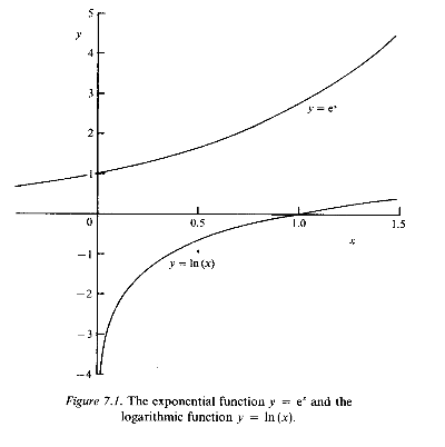
The graphs in Fig. 7.1 show how the functions exp (x) and ln (x) vary over a range of values of x. You can see that exp (x) is always positive, so that ln (x) is not defined for negative values of x.
From this definition and the differential equation for exp (x), it follows that if y = ln (x) then
![]()
This differential equation can be rearranged into a differential form which will arise several times during the forthcoming biological discussion:
![]()
When mathematicians come across this expression they recognize it as an old friend: it integrates to y = ln (x) + C, where C is an arbitrary constant (corresponding to the arbitrary multiple of exp (x) which we have already encountered).
Now we turn from calculus to algebra, and introduce a technique for simplifying certain expressions by the method of partial fractions. The biological models with which we shall be concerned sometimes require us to evaluate expressions similar to
![]()
The major complication here is the form of the denominator - which the method of partial fractions provides a way of simplifying. The aim is to calculate constants A and B which, for all values of x, satisfy the identity
![]()
If A and B exist, then we must have
![]()
and hence the numerators must be identical:
![]()
This identity can be maintained only if the coefficients of x and the constant terms on both sides are identical, which requires that
![]()
The constants A and B are determined from this pair of simultaneous equations to be A = 1 and B = - 1. Hence our original integral is simplified to

where C is the arbitrary constant of integration.
This digression into calculus and algebra should make clearer some of the mathematical manipulations of biological equations that follow.
Simple ideas about growth
The use of mathematics to describe the growth and decay of living organisms
interacting in a biological or ecological system requires some familiarity
with the exponential function et and its associated
differential equation to represent a quantity which grows with time t.
So first we look at a few ideas about growth and its description in mathematical
terms.
Consider, for example, the distance covered by a train travelling at 50mph from Glasgow to Manchester. In 1 hour it will have gone a distance of 50 miles, in 2 hours this will have increased to 100 miles, and so on - the distance s of the train from Glasgow increases steadily with the passage of time t (in hours) according to the formula
![]()
In more general terms, if the train's speed is u then the distance s depends on travel time t according to the relation
![]()
Such a relation describes the simplest kind of growth, in which the rate of increase is constant. The growth is then described as linear in time (because the graph of distance against time is a straight line, as we have seen in Chapters 1 and 6).
Although it may seem a little heavy-handed, it will suit our purpose to introduce here a little differential calculus. The velocity u, being the rate of change of distance with time, can be calculated as the derivative of s with respect to time t:
![]()
This is a differential equation - an equation involving derivatives which determines the rate of growth of distance with time.
A different type of growth is found when one considers the volume of a cube as a function of the length of its side. A box with side 1 m has a volume of 1 m3; doubling the side to 2 m increases the volume to 8 m3 and for a 3 m cube the volume is 27 m3. In this case, the growth of the volume V is related to the side length l by
![]()
This non-linear formula determines the volume as a function of the side length. It can be seen that increasing the side from 1 m to 2 m increases the volume by 7 m3 (from 1m3 to 8 m3); increasing the side from 2 m to 3 m increases the volume by 19 m3. Equal increases in the length do not yield equal increases in volume. This behaviour is a feature of non-linear relationships, and corresponds to the mathematical statement that the rate of change of volume with length of side depends on the length of side. The phrase 'rate of change' suggests that we can use differential calculus here. We know that if V and l are related by equation (7.15), then
![]()
This is a differential equation that determines the rate of growth of volume as a function of side length l.
We come now to a somewhat more complicated kind of growth, but one closer to the population dynamics we shall be discussing. Consider the sequence of numbers formed by starting with unity and doubling each time. These numbers form the sequence
![]()
Similarly, successive increase of each number by 50% generates the sequence 1, 1.5, 2.25, . . , (l.5)n. In general, if a is any positive number then the sequence an can be calculated and the numbers within it are said to grow exponentially. Consideration of such numbers leads us to generalize a little and discuss the features of a function y(x) defined by
![]()
where a is a real number greater than one, and x is real - positive or negative. A little experimenting with calculator, pencil and graph-paper will show that y(x) increases without limit as x increases positively, and decreases towards zero (becoming vanishingly small) as x decreases through negative values.
The feature of this type of growth which I want to stress is that the rate of growth of y; is proportional to y: the increase in y for unit increase in x is (a - l)y(x). The mathematical equation that describes such growth - one in which the rate of change of a quantity is proportional to the quantity itself - is
![]()
where k is a constant. The general solution of this equation is known to be -
![]()
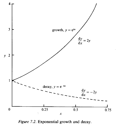
where A is an arbitrary constant; e we have met in equation (7.2). For example, it is easy to see that if k = 2 and y(x) = A e2x then dy/dx = 2Ae2x = 2y(x). The value of A is determined by specifying the value of y for some (single) specific value of x; usually we wish to start with a value of y when x = 0, corresponding to an initial condition which fixes the constant A. The differential equation in this case is said to describe exponential growth if k > 0; when k < 0 the solution y, decays steadily towards extinction (zero). This behaviour is shown in Fig. 7.2, with k = +2 and A = 1.
To summarize, we have discussed a variety of examples of growth, from linear to exponential systems, each of which has an associated differential equation. It will become clear that the concept of exponential growth has particular relevance to population dynamics.
Single-species population dynamics
The most commonly discussed mathematical models of a single biological population
are described by a differential equation which specifies the rate of change
(growth) of the population P(t) for a known growth rate R(P) as
follows:
![]()
This equation is to be solved for P as a function of time t, subject to an initial condition of the form P = P0 when t = 0. A particularly simple model of this kind is the so-called Malthusian or exponential growth described by
![]()
where k is the intrinsic growth rate per unit of the population. The solution of this linear differential equation is P = P0 ekt which grows without limit or decays to extinction depending on whether k is positive or negative, as shown in Fig. 7.2. This form of P(t) grows at a rate proportional to its current size, just as a sum of money does when invested in a bank or building society.
The intrinsic growth rate k is a parameter in the rather idealized biological growth system which equation (7.22) represents. We can think of it as defining the rate at which the population of a species might grow in the absence of any competition for or limitations on food. For example, if a small number of organisms are introduced to a large and suitable environment, they will tend to reproduce rapidly in line with the Malthusian rate. A remarkable example of this is known to have occurred with a species of fish, the striped bass. In about 1880, 435 of these fish were released into San Francisco Bay. Just twenty years later the commercial catch alone exceeded 550 tonnes - which suggests at least a millionfold increase over that period. A similarly explosive growth in the human species was foreseen by Malthus in the last century: Such an unrestricted increase of numbers in a population, however, is not sustained in practice because of limitations imposed by several factors, one of which is the finite food supply.
For many species living in a stable environment with a finite food supply, the population tends to a stable upper limit which depends on the environmental conditions. Below this limit, the environmental carrying capacity or saturation level, which we denote by L (positive), the population has an inherent or potential rate of growth which depends on the population size. Biological species, from microorganisms to mankind, are believed to be growth-limited in this fashion. A particular form of equation (7.21) matching such behaviour is a refinement of equation (7.22):
![]()
where k (>0) is the intrinsic or potential growth rate, achieved by the species for as long as its population is not large enough to strain the available food supply.
As a particular example of this general equation we take k = 2 and L = 1000. Then
![]()
This is a mathematical way of stating that at any particular moment the growth rate is 2 units per unit of population (say 1000 fish) per unit of time (a week say), but that in addition the fish population is limited to a maximum of 1000 by environmental constraints such as the availability of food. You can see that if the population P in equation (7.24) were to be greater than 1000, then the rate of growth would be negative and the population would decrease from such a value. This would happen if the owner of a fish farm overstocked his ponds in a misguided attempt to rear more fish.
The differential equation (7.24) can be solved by the method of partial fractions. To calculate the complete solution we must know how many fish there were to start with. If we assume there to have been 20, then it turns out that at a later time
![]()
Notice that this equation satisfies the condition P = 20 when t = 0. It also indicates that P approaches 1000 for large values of t, without ever actually reaching it. A graph of P as a function of time t is shown in Fig. 7.3. The greatest growth rate occurs when the graph is steepest, which is when dP/dt has its maximum value.
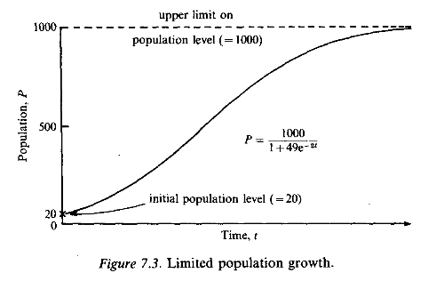
From equation (7.24) it follows that this will be when P[l - (P/ 1000)] is greatest; this is when P = 500.
There are two other starting values worth mentioning, because they give rise to steady population levels, unvarying with time. First, as is obvious, if the initial value of the population is zero then it will be zero for all later times; second, if it is initially 1000, then it will remain constant at this value. These unvarying solutions are called equilibrium states, and it is of interest to see what happens if, rather like prodding a tower of bricks, we disturb them a little to examine their stability.
First we examine the stability of the solution P = 1000. Suppose we perturb the population, by adding a small number p of population units to the existing 1000 units, so that P = l000 + p. Then, from equation (7.24) we have
![]()
The approximation is justified because p2/500 is very much smaller than p. This shows that p is proportional to e-2t, and so p will decay to nothing with the passage of time t; in other words, a slight disturbance to the population P = 1000 dies away and the level eventually returns to 1000. This stability therefore corresponds to that of a stable tower of bricks which sways slightly after being prodded, but soon returns to the vertical.
The equilibrium of the state P =0, however, is unstable. If P is small, say P = p, then equation (7.24) approximates to
![]()
and so p is proportional to e2t, which increases with time. Thus the disturbance grows in a way that corresponds to our tower of bricks swaying so much after being prodded that it falls over. The biological significance of this is that if we could exterminate this population completely it would remain extinct, but if we overlooked just a tiny population, capable of breeding, then the population would grow rapidly and re-establish the non-zero equilibrium state.
The influence of harvesting
In equations (7.23) and (7.24) the population P is influenced by its intrinsic
growth rate k and the carrying capacity L (the maximum population
size the environment can support). One reason for our mathematical modelling
of population growth is to get a better picture of the effect of man's predation
or harvesting of a particular species, for example by fishing for herring.
It is quite likely that the amount of harvesting through fishing will be
proportional to the fish population since, for example, if a trawler shoots
its nets into densely populated waters the catch will be greater than in
sparse waters. We can modify (7.23) to include the effect of such predation
by writing it as
![]()
where the constant F is the harvesting (fishing or culling) effort per unit of the population. With our previous figures of k = 2 and L = 1000, we have
![]()
which can be compared to equation (7.24) with the intrinsic growth rate reduced to 2 - F. Clearly, if F > 2 the population will eventually reduce to zero, and the species will become extinct through over-harvesting. However, if F < 2 then P will have a stable value when dP/dt =0. This value occurs with P = PS, where PS, the population level stable in the face of harvesting, satisfies the equation
![]()
that is, when
![]()
Compare this with the stable value of 1000 before we considered harvesting.
The harvested yield Y obtained from the population PS is FPS, and so
![]()
Thus Y is the sustainable yield, or fishing catch, corresponding to the fishing effort F. Obviously, as F increases then so does the size of the catch: if F is close to but less than 2, or close to but greater than zero, the yield Y is small. You can verify graphically or by using differential calculus that the largest yield will be obtained by adjusting fishing strategy and techniques so that F = 1, in which case the catch will be 500.
More generally, the optimum harvesting rate is k/2, where k is the intrinsic growth rate of the harvested species and the corresponding maximum sustainable yield is kL/4, where L is the environmental carrying capacity; any greater or lesser effort will lower the yield.
Of course, idealized analyses of the kind outlined here must not be taken too seriously by ecological planners. So many features of the real environment have been ignored including interactions with other species, and random fluctuations of the environment and in the distribution of species. Nevertheless, this example shows how potentially useful concepts can emerge from very simple models. Our results suggest that in order to determine the optimum harvesting effort, the intrinsic growth rate and the environmental carrying capacity of the target population should be found. These might form the basis of recommendations to a scientist or civil servant who is considering the advisability of allowing commercial fishing in a particular sea area.
A discrete approximation suggesting chaos
We approached our discussion of population growth, based on equation (7.23),
by using an exact mathematical analysis. This was possible only because our
model was a highly idealized one, and therefore highly simplified. Of course,
real systems are rather complicated and not amenable to such a precise analysis,
so only approximate (though very accurate) solutions can be obtained, by
numerical methods designed for use with a calculator or computer. For this
reason, and because of the interesting mathematical behaviour arising in
the process of approximation, we shall now look at numerical (or discrete)
approximations to equation (7.23).
There are many biological species, such as fruit flies and other crop pests, for which the population of one season lays eggs and then dies out; during the next season the eggs hatch and the population matures, and lays its eggs. The generations succeed one another season by season. Such a population, with non-overlapping generations, is well suited to study by ecologists. If we number the seasons 1, 2,... , n, . . . , the population in the nth season can be denoted by Pn As the population in one season is determined entirely by the population of the preceding season, then, in mathematical terms, Pn +1 is a function Pn .
In these seasonal populations there is a tendency for the population to increase from one generation to the next when it is small and to decrease when it is large; this instinctive form of population control is a response to a limited food supply. A mathematical expression for the dependence of Pn +1 on Pn, in this case is
![]()
A curve of the form y = 4lx( 1 - x) is called a parabola, and equation (7.33) states that the sequence of numbers Pn, it defines lie on such a curve.
We might well wonder what the numbers* Pn, actually look like, and it is not very difficult to investigate specific examples. For instance, suppose that l = ½ and start from n = 0 with P(0) = ¼.
Then, from equation (7.33), we can generate the sequence of numbers P0, P1, P2, . . . as follows:
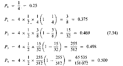
* Here P, is a fraction of some notional maximum population.
You can see that this sequence rapidly approaches a value (0.5) which remains unchanging from season to season (or generation to generation). As mathematicians we are inclined to ask why this happens in this instance, and whether it happens generally with any sequences generated by equation (7.33). The answer to this general question is 'No', but to discuss the topic further we need to go through some mathematical analysis.
First we note that equation (7.33), which defines Pn +1 in terms of a growth rate l and the population level Pn , of the preceding generation, possesses equilibrium points where Pn , does not change from one season to the next. In these circumstances Pn += Pn , and so this equilibrium value P satisfies a quadratic equation P = 4l P(l - P); it follows that P = 0 or P = 1 - 1/(4l).
Suppose that P is perturbed slightly from the equilibrium at P = 0, say to p, where pn is small. Then an approximate form of equation (7.33), using the small steps pn but ignoring the second power of pn, demonstrates that pn+1 = 4lpn. In other words, if 0 < 4l < 1, the perturbation decays away and P = 0 is a stable point, or attractor, of the system. If 4l > 1, this disturbance grows, the equilibrium is unstable and P = 0 is a called a repellor.
Similar analysis of the equilibrium at P = 1 - 1/(4l), perturbing by a small pn yields, to first order (i.e. ignoring powers of pn), the relation
![]()
If the successive perturbation steps pn are to decrease in absolute magnitude - which they will for a stable equilibrium in which the perturbation decays and P returns to its starting point - we require that - 1 < 2(1 - 2l) < 1, from which it follows that
![]()
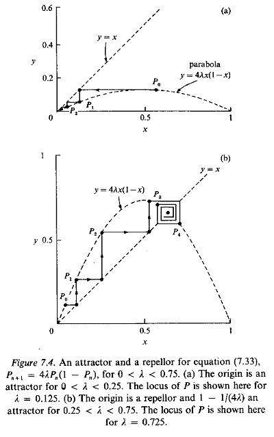
For these values of l the equilibrium is stable and P = I - 1/(4l) is an attractor; for all other values of l the equilibrium is locally unstable. The behaviour at successive steps can be illustrated graphically on a microcomputer; results obtained in this way are shown in Fig. 7.4, for l = 0.125 and l = 0.725.
We can also show from equation (7.33) that, if 0 < Pn, < 1 and 0 < l< 1, then 0 < Pn+1 < 1; the maximum occurs if Pn,=½ when Pn+1 = l (< 1). There is something interesting here because, although we would expect local stability only if 0 < l < ¾, this last conclusion has proved that the solutions Pn, will remain bounded (though presumably cycling in some fashion) if ¾< l < 1.
In view of this, it is tempting to investigate the behaviour of the sequence of Pn, steps defined by equation (7.33) as l increases from zero through ¾ to unity. We can simplify matters by concentrating on the behaviour of the equilibrium points at P = 0 and P = I - 1/(4l ) as the growth rate l is varied from zero to unity.
The transition from stable (attractor) to non-stable behaviour can be demonstrated easily using computer graphics. For values of l less than ¾, the population tends to either zero or P = 1- 1/(4l ), as illustrated in Fig. 7.4. When the growth rate l is increased above ¾, the population level no longer settles to a steady state.
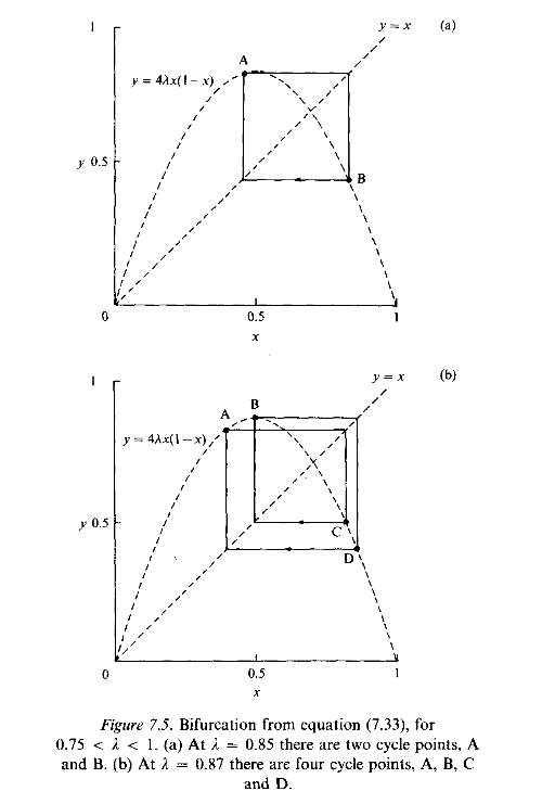
Instead it oscillates between a sequence of, at first, two values, and then, when l > 0.8624, four values - the population cycles through these values in successive seasons, as illustrated in Fig. 7.5. This splitting, or bifurcation, of the equilibrium continues through sequences of 8, 16,... , 2n, . . . points.
Beyond a critical value just above 0.89, the structure of the sequence becomes apparently irregular, and this region, where 0.892 < l < 1, is described as chaotic. The critical value of l is the limit of an infinite sequence of doublings with an infinity of attractors now associated with the cycling. The system behaves as no ordinary attractor - it is an example of what is called a strange attractor. You may find it surprising that a stepwise procedure, or iteration, based on a curve as simple as the parabola can give rise to such a rich variety and complexity of behaviour. It is fascinating to watch this complicated behaviour being generated graphically on a computer. All you need are a few lines of code to generate the steps according to equation (7.33), and the simplest of graphics showing the plot of pairs (Pn, Pn+1) on your screen for various values of l
Simple predator-prey systems
A limitation of the models we have considered so far is that they deal with
only a single species, and ignore competitive interaction with other species.
Now we look at the modelling of multi-specied populations by considering
systems in which one species is preyed on by another.
Consider an ecological system in which there are hunters who feed on prey, who themselves have an unlimited source of food; as an instance we might think of birds and earthworms. A simple but illustrative mathematical model can be constructed if we make a few (sweeping) assumptions:
- (1) If there were no hunters, the prey would grow without limit.
- (2) If there were no prey the hunters would eventually die out.
- (3) The rate at which the prey are captured is proportional to the product of the prey and the hunters - so that if the number of hunters or of prey increases, then so does the number of captured prey.
- (4) The rate at which the hunters increase in number is proportional to the product of the hunter and prey populations - so that if either the number of hunters or the availability of prey increases, then so does the number of hunter births.
A biological system with these properties can be represented by the following pair of equations, to be solved for the populations H and P:
![]()
Here the prey has an intrinsic growth rate, r, which would be achieved if there were no hunters, while the hunters would die away with an intrinsic death rate, s, in the absence of prey. The terms involving products of H and P, - aHP and bHP, define how the presence of hunters inhibits the growth of prey, while the presence of prey encourages the growth of hunters.
To make equations (7.37) more specific, suppose that a = 2, b = 1, r = 100 and s = 1000. Then
![]()
There are two equilibrium states for which dP/dt = dH/dt = 0.
You can check, if necessary by substituting the following values for P and H into equations (7.38), that these states are either
![]()
or
![]()
Suppose that the equilibrium (7.39) is slightly disturbed so that P = 1000 + p and H = 50 + h, where p and h are small. Then, approximately,
![]()
By taking the ratio of these equations, the variable t (time) drops out and we obtain the following relation between the small disturbances p and h:
![]()
This can be solved by the techniques of separating the derivative, giving
![]()
which in turn leads to
![]()
This is the equation of an ellipse, as shown in Fig. 7.6, and the value of the constant is determined by the values of p and h when the system is initially disturbed.
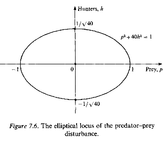
It is clear from this diagram, and from equation (7.44), that both p and h are restricted in value; p and h vary cyclically and the solution P = 1000 and H = 50 is stable in the sense that slight disturbances do not lead to violent, unrestricted variations - even though the variations are not damped out.
In similar fashion, we can look at the other equilibrium solution -extinction where both the prey and hunter populations P and H are zero (equation (7.40)). Now, with the assumed values of r = 100 and s = 1000, we find that small disturbances p and h from this extinction solution satisfy the equations
![]()
These yield p = Ae100t and h = Be-1000t, where A and B are the initial values of the p and h disturbances. These results show that the prey grows rapidly from zero while the hunters return to extinction: in other words, that extinction is an unstable equilibrium, with the prey achieving rapid growth in the absence of control by the hunters.
This model (based on equations (7.37)), though appealing to mathematicians, is considered unrealistic by most ecologists and biologists, mainly because of the undamped oscillations predicted by the ellipse shown in Fig. 7.6. In nature many cycles are observed, but their period and amplitude do not depend significantly on the initial conditions.They are determined primarily by system parameters such as growth rates and food supply,and usually tend to a stable state (or stable limit cycle) irrespective of the initial populations levels (see for example Fig 5.5 in Chapter 5). Even so, the model we have looked at provides useful insight into cycling and population collapse. Too many predators over-harvest their prey, causing a decline in the food supply; this is followed by a fall in the number of predators, leading to re-establishment of the prey and a subsequent rise of hunters - and so the wheel goes round and round.
Equilibrium states and limit cycles
The predator-prey system is unrealistic because perturbations to it give
rise to undamped cycling of the populations, determined totally by the starting
conditions. An interesting development of the basic predator-prey model is
obtained if we suppose that the growth of P, the number of prey, is
constrained by resources so that, even in the absence of hunters, there is
a limit on the prey population. With such a refinement the predator-prey
interactions are modified by the incorporation of an extra term (-
P/L) in the prey growth equation:
![]()
These equations represent a predator population H sustained by a prey population P which in turn is sustained by an environment with a prey-carrying capacity L. They might represent an ecosystem containing species of carnivore, herbivore and vegetation (such as foxes, rabbits and grass). By definition, the equilibrium points of this system are those for which dP/dt and dH/dt vanish simultaneously, so that both populations are steady. When the simultaneous equations (7.46) for P and H are solved with zero time-derivatives, we obtain
(1) P = 0 and H = 0.
(2) P = L and H = 0.
(3) P = s/b and H = (1 - Ls/b)r/a.
Although it is not a trivial task, we can examine the stability of these equilibrium solutions by examining the behaviour of small perturbations p and h about each of them in turn, as before. It can be shown that the total extinction of hunters and prey in state (1) is unstable. State (2) represents a condition in which there are no predators H, so the prey has reached the carrying capacity imposed by the environment; this turns out to be stable if and only if bL < s. Since we must have positive values for H and P, state (3) can be ignored unless bL > s; in fact state (3) is stable if and only if this inequality holds.
To sum up, we have shown that for this resource-limited form of the predator-prey model there are three steady states, one (and only one) of which is stable. Just which one it is depends on the system constants; the populations converge on state (2) if s < bL, and on state (3) otherwise. The total extinction of both hunters and prey -state (1) - is always unstable.
Models of this sort can be enhanced in various ways, for example by adding a component to represent harvesting by man of the predator, prey or both. Furthermore, there are forms of the growth rates which gives rise to stable limit cycles. The significance of a stable limit cycle is that it corresponds to a solution in which the populations cycle, as in Fig. 7.6, but the cycle does not depend on the initial population levels. This is a more acceptable view of cyclic behaviour in ecology than is provided by the simple model described in the last section, because ecologists believe nature to be influenced not so much by initial population levels as by the relationships between species in the system. Such models are often based on modifications of equations (7.46) in which the predator equation is of the form
![]()
This replacement represents the resource-limited growth of predator, the limitation being proportional to the density (P) of prey.
Concluding remarks
Our understanding of ecological system dynamics can be improved by the use
of matematical models based on simple but non-linear differential equations.
The mathematical and computational properties of these equations lead quickly
to topics of some sophistication, such as bifurcation, chaos and limit cycling.
The mathematical features depend on the types of non-linearity included in
the growth rates used in such models, and can be
effectively
followed by using the graphics facility of a microcomputer. Even very
simple computer programs can adequately illustrate the dynamical behaviour
of these systems.
I hope your imagination has been fired by the richness of behaviour exhibited by the illustrations given here; it is very easy to devise others. But herein lies a danger the mathematician must avoid falling into the trap of believing that complexity of modelling reflects the complexity of nature. Mathematical models are like metaphors: if taken too literally they lose their point. Population is only one aspect of an ecological system; others are age structure, genetics, mutation and climatic variations. Even so, as in so many fields of investigation, mathematics provides a powerful means for developing new insights into essentially complicated systems.
Further reading |
| D. R. Hofstadter, 'Metamagical themas', in Scientific American, Nov.1981. |
| R. M. May, Stability and Complexity in Model Ecosystems (Princeton University Press, 1973). |
| J. D. Murray, Nonlinear Differential Equation Models in Biology (Clarendon Press, 1977). |
| W. W. Sawyer, Mathematicians Delight (Penguin, 1943). |
| From: Lee Borrell <templarser@yahoo.co.uk>
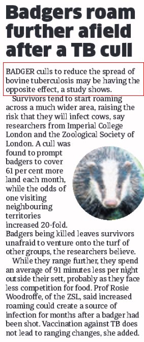
To: Susan Stewart <thepliedes@yahoo.co.uk> Sent: Thursday, 22 March 2012, 13:07 Subject: Re: grey squirrels With respect to speciesism,which is what culling is (we'd never tolerate it in humans,if we ethnically cleansed a race if they were a problem - and some are.). The attached shows that notables from the music industry are as incensed about such things as the layperson. The recent news that cetaceans were being considered for human rights,suggests all conservation includes the notion of animal rights. It doesn't make much sense if it doesn't. The mere fact that someone of Dappy's IQ can grasp what is noxious about the situation (unless he has been cranked into action by Brian May) suggests that culling is not something only conservation groups are taking action about,and it doesn't take a genius to respond. As it happens,I doubt Dappy is one of those who understands population dynamics - http://www.medlockandtame.org.uk/natnum2.html The simple fact is that a merely taking something out of the loop because it appears to be "a problem" lacks foresight and understanding of the interrelation of species. Not to mention the fact that it takes an arbitrary exception to a single species because of a perceived problem with knock on effects towards others. One cannot cherry pick which species is more important,especially in the case of the grey squirrel,it is exceptionally good at doing what nature wants - procreating and being a success. Because we apply human moral judgments to animal activity,it is found wanting,much as deer are for destroying trees or badgers for spreading TB (one wonders what seal pups have done). These are not "crimes" - they merely interfere with what humans think is right,just by the animal behaving normally.Management of the effects of one species upon another requires intelligence not a shotgun. Killing merely impacts that one species,and thence has unknown effects upon the rest of the various populations. Models such as those in the link show that counter-intuitive effects happen. If you think you are saving one species from another - think again- that is too simplistic.Take one "criminal" out of the loop,and like sharks teeth - 5 more may come along to fill the niche.
Culling is a simplistic and bombastic methodology that fails to understand the complexity of the web of life- if anyone cares to take exception,then explain to me what is wrong with the maths on the link,or at the very least explain to me why it is ethically sound to cull an animal but not to ethnically cleanse people,I think you will at least find you have double standards and are guilty of speciesism. 1. - The tragic fate of the fat caribou, or why we have to fear the reindeer of St Matthew more than the wolves of Wall-Street During World War II, the US Coast Guard decided to install long range aids to navigation in St Matthew Island, a remote rock in the Bering Sea in Alaska, and to stock emergency food source there. In August the same year, they released 29 reindeer (known as caribou in North America) on the island as a backup food source for the 19 men stationed there. As World War II drew to an end, the Coast Guard left the island and, by the same token, the population of reindeer growing unchecked as their only predators, the 19 men on duty there, were sent back home. It followed a dramatic boom & burst of population dynamics (figure 1). From 1944 to 1966 the number of these herbivores, which did not have to worry anymore about any predator and ate all the available lichen, increased from 29 to 6,000. In 1957, their body weight was found to exceed that of reindeer in domestic herds by 24.5 percent among females and 46.6 percent among males. Then, the following winter, as they faced a limited food supply to sustain their number and their massive body weight, they underwent a crash die-off, the population falling from 6,000 to 42 (figure 3).
THE HYDRA PARADOX GARDENERS who apply insecticide do not expect pest populations to flourish. Nor do fishery regulators anticipate that more fishing will boost the size of their stocks. Perhaps they should. Thanks to the complexity of the natural world, killing individuals doesn't always end up diminishing their population. The failure to consider this possibility could be confounding resource management and pest eradication, and perhaps even attempts to boost numbers of threatened species. A decade ago, my collaborator Hiroyuki Matsuda and I coined the term hydra effect to describe all situations where a higher death rate in a particular species ultimately increases the size of its population. We named this phenomenon after the multi-headed serpent of Greek myth that grew two heads for each one that Hercules cut off. The hydra effect is just one example of a more general phenomenon where adverse changes in the environment that reduce the growth ...
http://www.newscientist.com/article/mg22630232.700-hydra-paradox-when-culling-animals-makes-them-thrive.html
|

 .
.